hobrien.github.io

Tidyverse Tutorial

The Tidyverse is a collection of R packages for manipulating tidy data
They do not necessarily extend functionality beyond base R but they do make things easier and faster:
- consistent syntax (always snake_case, always take the data as the first argument)
- consistent output (type-stable, never makes assumptions about how you want to treat your data)
- amenable to piping
Compact data (AKA wide) vs tidy data (AKA long data):
compact:

GeneID	Sample1	Sample2
Gene1	473	526
Gene2	7203	6405
Gene3	59487	51467

wide:

GeneID	Sample	Count
Gene1	Sample1	473
Gene2	Sample1	7203
Gene3	Sample1	59487
Gene1	Sample2	526
Gene2	Sample2	6405
Gene3	Sample2	51467

Each variable you measure should be in one column.
Each different observation of that variable should be in a different row.
There should be one table for each “kind” of variable.
If you have multiple tables, they should include a column in the table that allows them to be linked.

The pipe function:

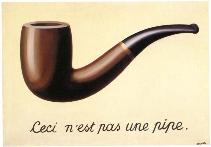
library(magrittr) #Ceci ne pas une pipe
set.seed(69)
rnorm(10) %>% mean

Ceci ne pas une pipe

tibble/readr

tibble is the tidyverse version of a dataframe
readr is the tidyverse version of read.delim
tibbles look nicer than dataframes when printed and are more consistent/predictable:
- “tibble() does much less than data.frame(): it never changes the type of the inputs (e.g. it never converts strings to factors!), it never changes the names of variables, it only recycles inputs of length 1, and it never creates row.names()”
- when printed to the screen, tibbles only display 10 rows and as many columns as can fit on
- they also display the data type of each column and the dimensions of the dataframe
readr creates tibbles. It’s also fast and flexible
if a column of mixed numbers and strings is coearsed using as.numeric(), traditional dataframes will return the rank of the factor levels, rather than the numbers:

df <- read.delim("examples/SampleInfo.txt")
2 * as.numeric(df$ReadLength)
# [1] 6 6 6 6 6 6 6 8 4 6 6 4 2 4 4 2 2 6 4 2 2 4 4 2 4 4 2...

2 * as.numeric(as.character(df$ReadLength))
# [1] 152 152 152 152 152 152 152  NA 250 152 152 250 200

tibble <- read_tsv("examples/SampleInfo.txt")
2 * as.numeric(tibble$ReadLength)
# [1] 152 152 152 152 152 152 152  NA 250 152 152 250 200

tidyr

tidyr converts between wide and long formats
it can also split a column into multiple columns

wide <-tribble(
  ~Gene, ~Sample1,  ~Sample2,
  "Gene1_APOE1", 473,  526,
  "Gene2_SETD1A", 7203,  6405,
  "Gene3_TCF4", 59487, 51467
)

long <- gather(tibble, Sample, Value, -Gene)
wide <- spread(long, Sample, Value)

separate(wide, Gene, c("GeneID", "Gene_name"))

dplyr

dplyr is for dataframe/tibble manipulation
- filtering rows (filter)
- selecting columns (select)
- modifying columns (mutate)
- joining tables (left_join, right_join, full_join, inner_join)
- summarise columns (summarise)
- group-wise summaries (group_by)
Select columns

head(tibble[,c('Sample', 'Sex')])
select(SchoolData, Sample, Sex) %>% head

Select rows

head(subset(tibble, PCW< 14))
filter(tibble, PCW<14) %>% head

Sort

head(tibble[order(tibble$RIN),])
arrange(tibble, RIN) %>% head

Calculate group means

head(aggregate(PCW ~ Sex, data=tibble, FUN=function(x) av_score=mean(x)))
#I can't figure out how to rename the output
tibble %>% group_by(Sex) %>% summarise(av_age=mean(PCW)) %>% head

Calculate multiple stats

head(aggregate(RIN ~ Sex+PCW, data=tibble, FUN=function(x) c(mean=mean(x), var=var(x))))
tibble %>% group_by(Sex, PCW) %>% summarise(mean=mean(RIN), var=var(RIN)) %>% head

Count occurences per group

head(aggregate(RIN ~ Sex, data=tibble,  FUN=function(x) num_students=length(x)))
tibble %>% group_by(Sex) %>% summarise(num_samples=n()) %>% head

Compute new values

tibble$total_length <- 2 * as.numeric(tibble$ReadLength)
head(SchoolData)
tibble %>% mutate(total_length=2 * as.numeric(ReadLength)) %>% head

Pipe results to ggplot

library(ggplot2)

tibble %>% 
    group_by(Sex) %>% 
    summarise(mean=mean(PCW), se=sd(PCW)/sqrt(n())) %>% 
    ggplot(aes(x=Sex, y=mean)) +
        geom_bar(stat="identity", fill="royalblue4", alpha=1/2) +
        geom_errorbar(aes(ymin=mean-se, ymax=mean+se), colour="royalblue4", alpha=1/2)

Incorporate other datasets

tibble %>% 
    group_by(Sex) %>% 
    summarise(mean=mean(PCW), se=sd(PCW)/sqrt(n())) %>% 
    ggplot(aes(x=Sex, y=mean)) +
        geom_jitter(aes(x=Sex, y=PCW), alpha=1/10, 
                    position = position_jitter(width = 0.2), 
                    colour="royalblue4", data=tibble) +
        geom_point(stat="identity", alpha=2/3, shape=5, size=2, colour="royalblue4") +
        geom_errorbar(aes(ymin=mean-se, ymax=mean+se), colour="royalblue4", alpha=2/3)

Select the highest RIN sample for each age
- multiple results if tied; use row_number() if you want a single sample per age

tibble %>% group_by(PCW) %>% filter(min_rank(desc(RIN)) == 1)

Calculate deviation from sex-specific mean age for each sample

tibble %>% 
    group_by(Sex) %>% 
    mutate(mean = mean(PCW)) %>% 
    ungroup() %>% 
    mutate(deviation=PCW-mean)

Combine dataframes
- works the same as merge, but a lot faster

counts<-read_tsv("Counts.txt")

inner_join(tibble, counts, by=c("Sample" = "SampleID")) # keeps only rows common to both datasets
left_join(tibble, counts, by=c("Sample" = "SampleID")) #keeps all rows in left dataframe, adding NA when row is missing from right dataset
right_join(tibble, counts, by=c("Sample" = "SampleID")) #keeps all rows in right, adding NA when row is missing from left dataset
full_join(tibble, counts, by=c("Sample" = "SampleID")) #keeps all rows in both, adding NA when row is missing from either dataset

stringr

package for string manipulation
extract fragment size estimate from homer peak calling

frag_size <- read_file("examples/peak_calling.txt") %>%
    str_extract("(?<=fragment size = )\\d+") %>% 
    as.numeric()

purrr

tidy version of the apply family
apply a function across subsets of a data frame (among other things)
correlate RIN vs mapping stats

inner_join(tibble, counts, by=c("Sample" = "SampleID")) %>%
    gather(stat, value, 7:13) %>%
    group_by(stat) %>%
    nest() %>%
    mutate(cor=map(data, ~cor.test(RIN, .$value)), r=map_dbl(cor, 4), p=map_dbl(cor, 3)) %>%
    select(-data, -cor)

Useful resources

Alternatives to dplyr

ddply{plyr} (slow)
data.table (confusing)

This site is open source. Improve this page.